Simulation 7 break down
Changes
Significant fitness function tuning.
Results
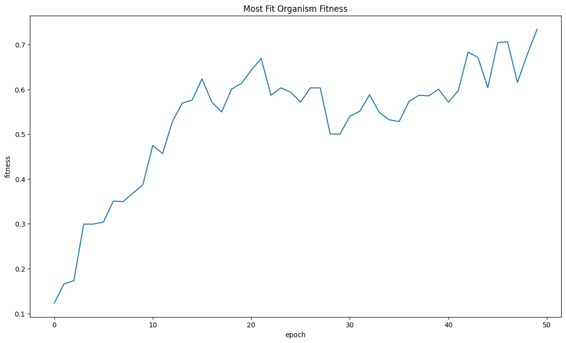
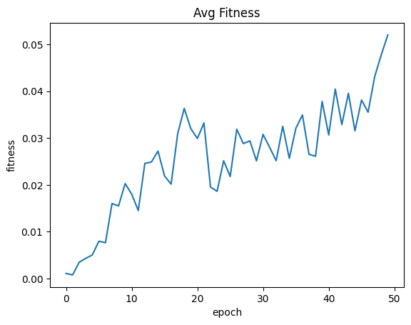
We finally got trees!! This was the main goal for Project Genesis. The average fitness was still trending upwards by the 50th epoch.
1
2
3
4
5
6
7
8
9
10
11
12
13
14
15
16
17
18
19
20
21
22
23
24
25
26
27
28
29
30
31
32
33
34
35
36
| import pandas as pd
import json
import seaborn as sns
import matplotlib.pyplot as plt
import math
import gzip
import os
def compareAvgMetricsByEpoch(dataframe, firstColumn, secondColumn ):
avgFirstColumnDf = dataframe.groupby('epoch', as_index=False)[firstColumn].mean()
avgSecondColumnDf = dataframe.groupby('epoch', as_index=False)[secondColumn].mean()
joinedData = pd.merge(avgFirstColumnDf, avgSecondColumnDf, on='epoch')
avgEpochOverlay = joinedData.melt(id_vars='epoch', var_name='Metric', value_name='Value')
return sns.lineplot(data=avgEpochOverlay, x='epoch', y='Value', hue='Metric')
def read_files_to_dataframe(basedirectory, metric):
dataframes = []
for directory in os.listdir(basedirectory):
if( directory != 'overview.json' ):
filepath = os.path.join(os.path.join(basedirectory, directory), metric + '.txt.gz')
with gzip.open(filepath, 'rb') as f:
df = pd.read_json(f,lines=True)
df['epoch'] = int(directory.rsplit('-', 1)[-1])
dataframes.append(df)
return pd.concat(dataframes, ignore_index=True)
def readPopulationOverTime(file):
raw_df = pd.read_json(file)
overview = pd.json_normalize(raw_df['worlds'])
overview['epoch'] = overview['name'].str.split('-', expand=True)[2].astype(int)
trimmed = pd.DataFrame(overview, columns=['epoch', 'totalOrganisms'])
return trimmed.iloc[::2]
|
Global Variable:
1
2
3
4
| INPUT_FILE_DIR = '/Users/luke/dev/analysis/data/simulation98'
METRIC='Performance'
EXPANDED_FITNESS_MAGNIFICATION = { 'startIndex': 0, 'count': 50 }
|
Global Computed Variables:
1
2
| fullSimulationDataDf = read_files_to_dataframe( INPUT_FILE_DIR, METRIC)
populationOverTimeDf = fullSimulationDataDf.value_counts('epoch').reset_index(name='totalOrganisms')
|
Analysis:
1
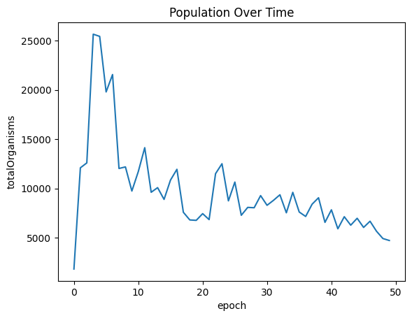
| sns.lineplot(x="epoch", y="totalOrganisms", data=populationOverTimeDf ).set_title("Population Over Time")
|
1
| Text(0.5, 1.0, 'Population Over Time')
|
1
2
3
| mostFitByEpochDf = fullSimulationDataDf.groupby('epoch')['fitness'].max().reset_index()
plt.figure(figsize=(14, 8))
sns.lineplot(x="epoch", y="fitness", data=mostFitByEpochDf ).set_title("Most Fit Organism Fitness")
|
1
| Text(0.5, 1.0, 'Most Fit Organism Fitness')
|
1
2
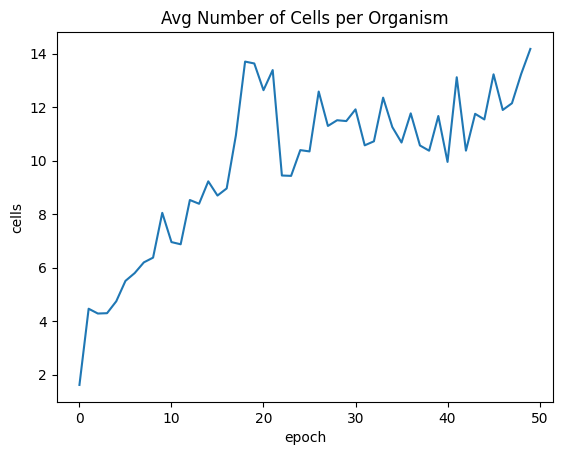
| avgSizeByEpoch = fullSimulationDataDf.groupby('epoch', as_index=False)['cells'].mean()
sns.lineplot(x="epoch", y="cells", data=avgSizeByEpoch ).set_title("Avg Number of Cells per Organism")
|
1
| Text(0.5, 1.0, 'Avg Number of Cells per Organism')
|
1
2
3
4
5
6
7
8
9
10
11
12
13
14
15
16
17
18
19
20
21
22
23
24
25
26
27
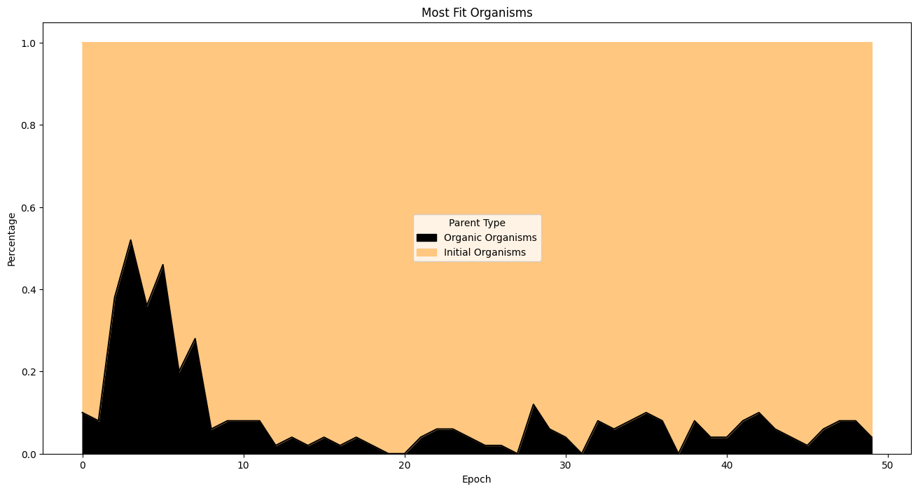
| fitnessHeritage = (
fullSimulationDataDf.sort_values(by='fitness', ascending=False)
.groupby('epoch')
.head(50)
)
percentages = (
fitnessHeritage.assign(
isOrigOrganism =fitnessHeritage['parentId'].eq('GOD')
)
.groupby('epoch')['isOrigOrganism']
.value_counts(normalize=True)
.unstack(fill_value=0)
.rename(columns={True: 'Initial Organisms', False: 'Organic Organisms'})
)
percentages.plot(
kind='area',
stacked=True,
figsize=(16, 8),
colormap='copper',
title='Most Fit Organisms'
)
plt.ylabel('Percentage')
plt.xlabel('Epoch')
plt.legend(title='Parent Type')
plt.show()
|
1
2
| avgFitnessByEpoch = fullSimulationDataDf.groupby('epoch', as_index=False)['fitness'].mean()
sns.lineplot(x="epoch", y="fitness", data=avgFitnessByEpoch ).set_title("Avg Fitness")
|
1
| Text(0.5, 1.0, 'Avg Fitness')
|
1
2
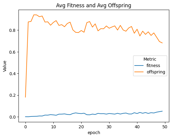
| linePlt = compareAvgMetricsByEpoch(fullSimulationDataDf, 'fitness', 'offspring')
nothing = linePlt.set_title('Avg Fitness and Avg Offspring')
|
1
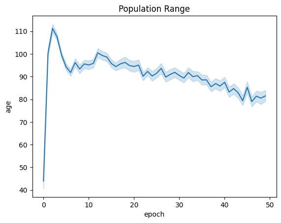
| linePlt = sns.lineplot(x="epoch", y="age", data=fullSimulationDataDf ).set_title("Population Range")
|
1
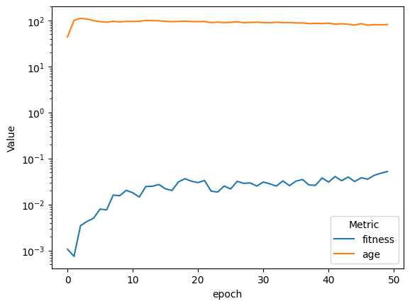
| compareAvgMetricsByEpoch(fullSimulationDataDf, 'fitness', 'age').set_yscale('log')
|
1
2
3
4
5
6
7
8
9
10
11
12
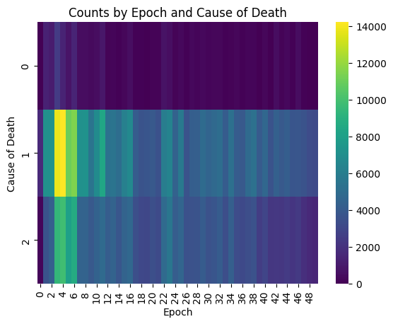
| trend = (
fullSimulationDataDf.groupby(['epoch', 'causeOfDeath'])
.size()
.reset_index(name='count')
.pivot(index='epoch', columns='causeOfDeath', values='count')
.fillna(0)
)
sns.heatmap(trend.T, cmap="viridis", annot=False, fmt="g")
plt.xlabel("Epoch")
plt.ylabel("Cause of Death")
plt.title("Counts by Epoch and Cause of Death")
plt.show()
|
Death value key is Unknown (0), Stagnation (1), Exhaustion (2), OldAge (3);
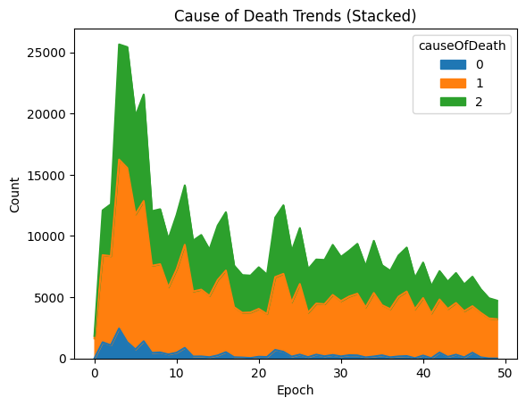
1
2
3
4
5
| trend.plot.area()
plt.xlabel("Epoch")
plt.ylabel("Count")
plt.title("Cause of Death Trends (Stacked)")
plt.show()
|